{
"info": {
"author": "Tirthajyoti Sarkar",
"author_email": "tirthajyoti@gmail.com",
"bugtrack_url": null,
"classifiers": [
"Development Status :: 4 - Beta",
"Intended Audience :: Developers",
"Intended Audience :: Education",
"Intended Audience :: Financial and Insurance Industry",
"Intended Audience :: Healthcare Industry",
"Intended Audience :: Information Technology",
"Intended Audience :: Science/Research",
"License :: OSI Approved :: GNU General Public License v3 or later (GPLv3+)",
"Operating System :: OS Independent",
"Programming Language :: Python",
"Programming Language :: Python :: 3.5",
"Programming Language :: Python :: 3.6",
"Programming Language :: Python :: 3.7",
"Topic :: Education",
"Topic :: Scientific/Engineering",
"Topic :: Scientific/Engineering :: Information Analysis",
"Topic :: Scientific/Engineering :: Mathematics",
"Topic :: Software Development",
"Topic :: Software Development :: Libraries",
"Topic :: Software Development :: Libraries :: Python Modules",
"Topic :: Utilities"
],
"description": "# mlr (`pip install mlr`)\n\n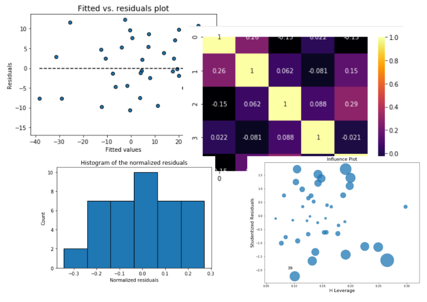\n\nA lightweight, easy-to-use Python package that combines the `scikit-learn`-like simple API with the power of **statistical inference tests**, **visual residual analysis**, **outlier visualization**, **multicollinearity test**, found in packages like `statsmodels` and R language.\n\nAuthored and maintained by **Dr. Tirthajyoti Sarkar ([Website](https://tirthajyoti.github.io), [LinkedIn profile](https://www.linkedin.com/in/tirthajyoti-sarkar-2127aa7/))**\n\n### Useful regression metrics,\n* MSE, SSE, SST \n* R^2, Adjusted R^2\n* AIC (Akaike Information Criterion), and BIC (Bayesian Information Criterion)\n\n### Inferential statistics,\n* Standard errors\n* Confidence intervals\n* p-values \n* t-test values \n* F-statistic\n\n### Visual residual analysis,\n* Plots of fitted vs. features, \n* Plot of fitted vs. residuals, \n* Histogram of standardized residuals\n* Q-Q plot of standardized residuals\n\n### Outlier detection\n* Influence plot\n* Cook's distance plot\n\n### Multicollinearity\n* Pairplot\n* Variance infletion factors (VIF)\n* Covariance matrix\n* Correlation matrix\n* Correlation matrix heatmap\n\n## Requirements\n\n* numpy (`pip install numpy`)\n* pandas (`pip install pandas`)\n* matplotlib (`pip install matplotlib`)\n* seaborn (`pip install seaborn`)\n* scipy (`pip install scipy`)\n* statsmodels (`pip install statsmodels`)\n\n## Install\n\n(On Linux and Windows) You can use ``pip``\n\n```pip install mlr```\n\n(On Mac OS), first install pip,\n```\ncurl https://bootstrap.pypa.io/get-pip.py -o get-pip.py\npython get-pip.py\n```\nThen proceed as above.\n\n---\n\n## Quick Start\n\nImport the `MyLinearRegression` class,\n\n```\nfrom MLR import MyLinearRegression as mlr\nimport numpy as np\n```\n\nGenerate some random data\n\n```\nnum_samples=40\nnum_dim = 5\nX = 10*np.random.random(size=(num_samples,num_dim))\ncoeff = np.array([2,-3.5,1.2,4.1,-2.5])\ny = np.dot(coeff,X.T)+10*np.random.randn(num_samples)\n```\n\nMake a model instance,\n\n```\nmodel = mlr()\n```\n\nIngest the data\n\n```\nmodel.ingest_data(X,y)\n```\n\nFit,\n\n```\nmodel.fit()\n```\n---\n\n## Directly read from a Pandas DataFrame\nYou can read directly from a Pandas DataFrame. Just give the features/predictors' column names as a list and the target column name as a string to the `fit_dataframe` method.\n\nAt this point, only numerical features/targets are supported but in future releases we will support categorical variables too. \n\n```\n<... obtain a Pandas DataFrame by some processing>\ndf = pd.DataFrame(...)\nfeature_cols = ['X1','X2','X3']\ntarget_col = 'output'\n\nmodel = mlr()\nmodel.fit_dataframe(X=feature_cols,y = target_col,dataframe=df)\n```\n\n---\n\n## Metrics\nSo far, it looks similar to the linear regression estimator of Scikit-Learn, doesn't it?\n
Here comes the difference,\n\n### Print all kinds of regression model metrics, one by one,\n\n```\nprint (\"R-squared: \",model.r_squared())\nprint (\"Adjusted R-squared: \",model.adj_r_squared())\nprint(\"MSE: \",model.mse())\n\n>> R-squared: 0.8344327025902752\n Adjusted R-squared: 0.8100845706182569\n MSE: 72.2107655649954\n\n```\n\n### Or, print all the metrics at once!\n\n```\nmodel.print_metrics()\n\n>> sse: 2888.4306\n sst: 17445.6591\n mse: 72.2108\n r^2: 0.8344\n adj_r^2: 0.8101\n AIC: 296.6986\n BIC: 306.8319\n```\n---\n\n## Correlation matrix, heatmap, covariance\n\nWe can build the correlation matrix right after ingesting the data. This matrix gives us an indication how much multicollinearity is present among the features/predictors.\n\n### Correlation matrix\n```\nmodel.ingest_data(X,y)\nmodel.corrcoef()\n\n>> array([[ 1. , 0.18424447, -0.00207883, 0.144186 , 0.08678109],\n [ 0.18424447, 1. , -0.08098705, -0.05782733, 0.19119872],\n [-0.00207883, -0.08098705, 1. , 0.03602977, -0.17560097],\n [ 0.144186 , -0.05782733, 0.03602977, 1. , 0.05216212],\n [ 0.08678109, 0.19119872, -0.17560097, 0.05216212, 1. ]])\n```\n\n### Covariance\n\n```\nmodel.covar()\n\n>> array([[10.28752086, 1.51237819, -0.01770701, 1.47414685, 0.79121778],\n [ 1.51237819, 6.54969628, -0.5504233 , -0.47174359, 1.39094876],\n [-0.01770701, -0.5504233 , 7.05247111, 0.30499622, -1.32560195],\n [ 1.47414685, -0.47174359, 0.30499622, 10.16072256, 0.47264283],\n [ 0.79121778, 1.39094876, -1.32560195, 0.47264283, 8.08036806]])\n```\n\n### Correlation heatmap\n\n```\nmodel.corrplot(cmap='inferno',annot=True)\n```\n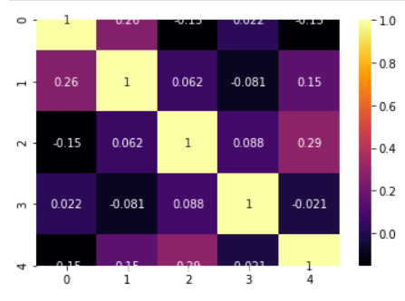\n\n## Statistical inference\n\n### Perform the F-test of overall significance\nIt retunrs the F-statistic and the p-value of the test. \n\nIf the p-value is a small number you can reject the Null hypothesis that all the regression coefficient is zero. That means a small p-value (generally < 0.01) indicates that the overall regression is statistically significant.\n```\nmodel.ftest()\n\n>> (34.270912591948814, 2.3986657277649282e-12)\n```\n\n### How about p-values, t-test statistics, and standard errors of the coefficients?\nStandard errors and corresponding t-tests give us the p-values for each regression coefficient, which tells us whether that particular coefficient is statistically significant or not (based on the given data).\n\n```\nprint(\"P-values:\",model.pvalues())\nprint(\"t-test values:\",model.tvalues())\nprint(\"Standard errors:\",model.std_err())\n\n>> P-values: [8.33674608e-01 3.27039586e-03 3.80572234e-05 2.59322037e-01 9.95094748e-11 2.82226752e-06]\n t-test values: [ 0.21161008 3.1641696 -4.73263963 1.14716519 9.18010412 -5.60342256]\n Standard errors: [5.69360847 0.47462621 0.59980706 0.56580141 0.47081187 0.5381103 ]\n\n```\n\n### Confidence intervals\n```\nmodel.conf_int()\n\n>> array([[-10.36597959, 12.77562953],\n [ 0.53724132, 2.46635435],\n [ -4.05762528, -1.61971606],\n [ -0.50077913, 1.79891449],\n [ 3.36529718, 5.27890687],\n [ -4.10883113, -1.92168771]])\n\n```\n\n## Visual analysis of the residuals\nResidual analysis is crucial to check the assumptions of a linear regression model. `mlr` helps you check those assumption easily by providing straight-forward visual analytis methods for the residuals.\n\n### Fitted vs. residuals plot\nCheck the assumption of constant variance and uncorrelated features (independence) with this plot\n```\nmodel.fitted_vs_residual()\n```\n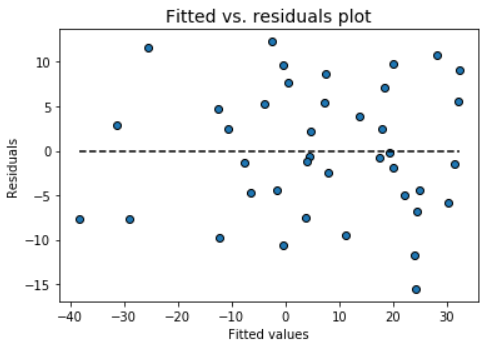\n\n### Fitted vs features plot\nCheck the assumption of linearity with this plot\n```\nmodel.fitted_vs_features()\n```\n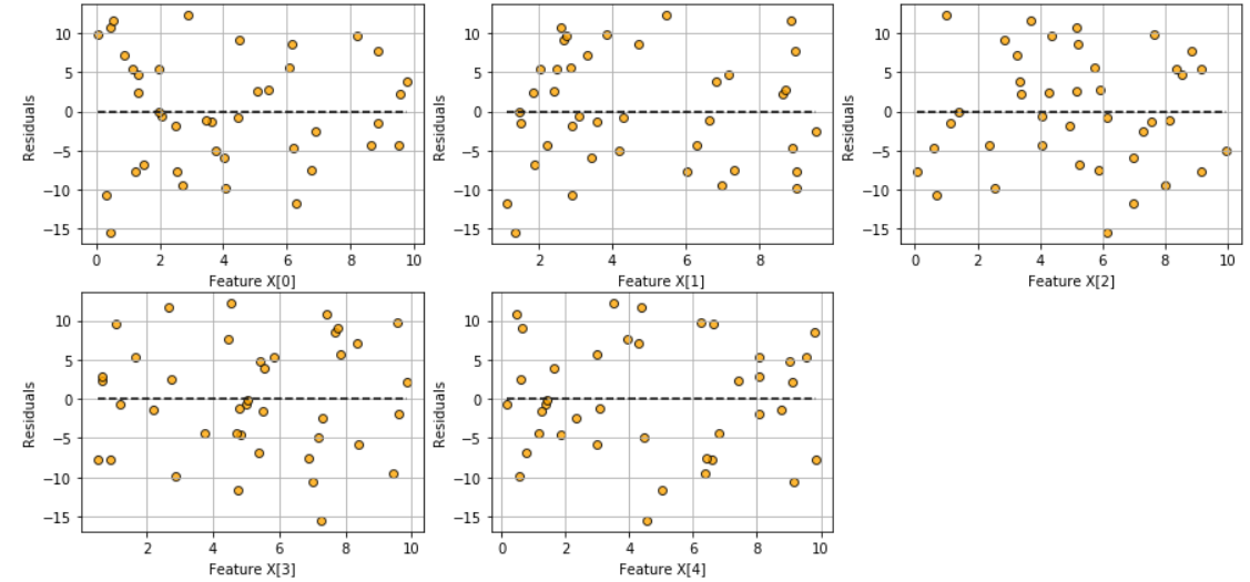\n\n### Histogram and Q-Q plot of standardized residuals\nCheck the normality assumption of the error terms using these plots,\n```\nmodel.histogram_resid()\n```\n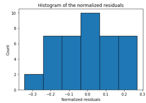\n
\n```\nmodel.qqplot_resid()\n```\n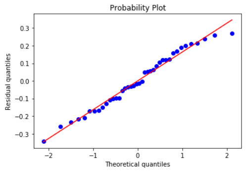\n\n## Do more\n\nDo more fun stuff with your regression model.\nMore features will be added in the future releases!\n\n* Outlier detection and plots\n* Multicollinearity checks\n\n\n\n",
"description_content_type": "text/markdown",
"docs_url": null,
"download_url": "",
"downloads": {
"last_day": -1,
"last_month": -1,
"last_week": -1
},
"home_page": "https://github.com/tirthajyoti/mlr",
"keywords": "Regression,Linear regression,Data science,Machine learning,Engineering,Statistics,Modeling,Analytics,Predictive analytics,Data mining",
"license": "GPLv3+",
"maintainer": "",
"maintainer_email": "",
"name": "mlr",
"package_url": "https://pypi.org/project/mlr/",
"platform": "",
"project_url": "https://pypi.org/project/mlr/",
"project_urls": {
"Homepage": "https://github.com/tirthajyoti/mlr"
},
"release_url": "https://pypi.org/project/mlr/0.1.0/",
"requires_dist": [
"numpy",
"pandas",
"matplotlib",
"seaborn",
"statsmodels"
],
"requires_python": "",
"summary": "Linear regression utility with inference tests, residual analysis, outlier visualization, multicollinearity test, and other features",
"version": "0.1.0"
},
"last_serial": 5622423,
"releases": {
"0.1.0": [
{
"comment_text": "",
"digests": {
"md5": "e7c592f0c31ef79d2a5ceb19f58d0f3f",
"sha256": "53bc44caa5f68582949654b42d52557eb06ea4d677bc9a954ea8a9f0d8b04a65"
},
"downloads": -1,
"filename": "mlr-0.1.0-py3-none-any.whl",
"has_sig": false,
"md5_digest": "e7c592f0c31ef79d2a5ceb19f58d0f3f",
"packagetype": "bdist_wheel",
"python_version": "py3",
"requires_python": null,
"size": 24194,
"upload_time": "2019-08-02T07:31:27",
"url": "https://files.pythonhosted.org/packages/64/aa/5877ade58c2d0b531e848ceae9d4bfa677b9df91932b7d3ef14e127ffa9e/mlr-0.1.0-py3-none-any.whl"
},
{
"comment_text": "",
"digests": {
"md5": "1857650eb14267992a0fb7ef8ef14ad0",
"sha256": "6d84592c3090efa37e762c1938e05faa102c992d5121b9ad92b77e06d72a8732"
},
"downloads": -1,
"filename": "mlr-0.1.0.tar.gz",
"has_sig": false,
"md5_digest": "1857650eb14267992a0fb7ef8ef14ad0",
"packagetype": "sdist",
"python_version": "source",
"requires_python": null,
"size": 13052,
"upload_time": "2019-08-02T07:31:30",
"url": "https://files.pythonhosted.org/packages/06/e6/23e5bc9d461e0eacb37fa63644bc5f0345ba2b7c4f76467477c2edbabcf7/mlr-0.1.0.tar.gz"
}
]
},
"urls": [
{
"comment_text": "",
"digests": {
"md5": "e7c592f0c31ef79d2a5ceb19f58d0f3f",
"sha256": "53bc44caa5f68582949654b42d52557eb06ea4d677bc9a954ea8a9f0d8b04a65"
},
"downloads": -1,
"filename": "mlr-0.1.0-py3-none-any.whl",
"has_sig": false,
"md5_digest": "e7c592f0c31ef79d2a5ceb19f58d0f3f",
"packagetype": "bdist_wheel",
"python_version": "py3",
"requires_python": null,
"size": 24194,
"upload_time": "2019-08-02T07:31:27",
"url": "https://files.pythonhosted.org/packages/64/aa/5877ade58c2d0b531e848ceae9d4bfa677b9df91932b7d3ef14e127ffa9e/mlr-0.1.0-py3-none-any.whl"
},
{
"comment_text": "",
"digests": {
"md5": "1857650eb14267992a0fb7ef8ef14ad0",
"sha256": "6d84592c3090efa37e762c1938e05faa102c992d5121b9ad92b77e06d72a8732"
},
"downloads": -1,
"filename": "mlr-0.1.0.tar.gz",
"has_sig": false,
"md5_digest": "1857650eb14267992a0fb7ef8ef14ad0",
"packagetype": "sdist",
"python_version": "source",
"requires_python": null,
"size": 13052,
"upload_time": "2019-08-02T07:31:30",
"url": "https://files.pythonhosted.org/packages/06/e6/23e5bc9d461e0eacb37fa63644bc5f0345ba2b7c4f76467477c2edbabcf7/mlr-0.1.0.tar.gz"
}
]
}